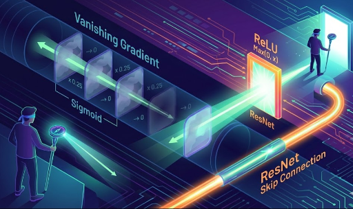
Vanishing Gradient: Why Deep Learning Suffers from Short‑Term Memory Loss
1. Introduction: "Boss, I can’t hear you!"

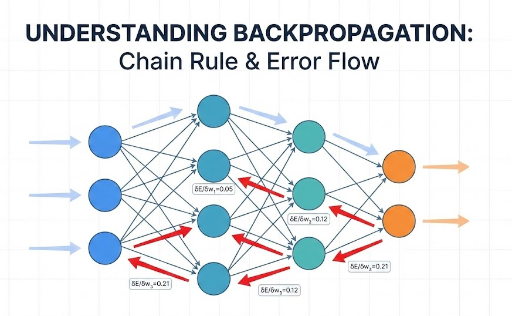
Last time we learned that backpropagation sends the loss from the output layer back to the input layer during training. In theory, deeper networks should solve more complex problems.
However, until the early 2000s deep learning was a dark age. Adding 10 or 20 layers often reduced performance or stopped training altogether.
It looks like this:
- CEO (output layer): "Hey! Why is the product quality so bad? (Loss occurs)"
- Executives → Managers → Supervisors…: The signal should travel downwards.
- Newbie (input layer): "…? What did they say? I heard nothing!"
The parameters at the front end, which handle the most critical groundwork, never get updated. That’s the vanishing gradient problem.
2. Root Cause: The Culprit is Sigmoid and Multiplication
Why does the signal disappear? It’s due to the sigmoid activation function and the chain rule’s inevitable mathematical properties.
(1) Sigmoid’s Betrayal: "A Tight Filter"
Early researchers loved sigmoid because it outputs values between 0 and 1, resembling a neuron’s firing probability. From a developer’s view, sigmoid is a compressor that squashes inputs.
- Problem 1: Gradient Ceiling (Max Gradient = 0.25)
- Differentiating the sigmoid shows a maximum derivative of only 0.25 (at x = 0).
- As soon as the input deviates slightly, the gradient approaches 0.
- Think of it as a mic volume set to the lowest level – no matter how loud you shout, only a whisper gets through.
(2) The Chain Rule Tragedy: "0.25 to the Nth Power"
Training updates weights as w = w - (learning_rate * gradient). Backpropagation multiplies derivatives from the output to the input.
Assume 30 layers. Even if every derivative is the maximum 0.25, the product is:
0.25 × 0.25 × … × 0.25 (30 times) ≈ 8×10⁻¹⁹
- Result: The gradient near the input is smaller than the machine’s precision, effectively zero.
- Effect: The weight update becomes
w = w - 0, so learning stalls. - Analogy: It’s like a network with 99.99% packet loss – error logs never reach the front‑end servers.
3. Solution 1: ReLU – "Going Digital"
The hero that solved this was a simple line of code: ReLU (Rectified Linear Unit).
When Professor Geoffrey Hinton’s team introduced it, everyone was shocked at its simplicity.
(1) Gradient Revolution: "1 or 0"
ReLU’s implementation:
def relu(x):
    return max(0, x)
Its derivative is clear:
- x > 0 (active): gradient = 1.
- x ≤ 0 (inactive): gradient = 0.
Why does this matter? In the positive region, multiplying by 1 never shrinks the signal.
1 × 1 × 1 × … × 1 = 1
Sigmoid would have eaten 0.25 each time; ReLU passes the signal losslessly.
(2) Performance Boost: exp() vs if
Sigmoid uses exp(x), a costly operation on CPU/GPU. ReLU is just a comparison (if x > 0), orders of magnitude faster.
(3) Caveat: Dying ReLU
If the input is negative, the gradient is 0, causing the neuron to die permanently. Variants like Leaky ReLU give a tiny slope for negative inputs.
4. Solution 2: ResNet (Residual Connections) – "A Dedicated Hotline"
ReLU allowed us to stack 20–30 layers, but ambition pushed us to 100 or 1000 layers, and training again failed. Enter ResNet (Residual Network).
(1) Idea: "Learn Only the Change"
Traditional nets try to produce the entire output H(x) from input x. ResNet’s skip connection changes the equation:
Output = F(x) + x
It tells the model: You only need to learn the residual (difference) from the input; the original stays intact.
(2) Gradient Superhighway
In backpropagation, addition distributes over differentiation:
∂Output/∂x = ∂F(x)/∂x + 1
The +1 guarantees that even if ∂F(x)/∂x vanishes, at least a unit gradient survives and reaches the front end.
- Without ResNet: A blocked gradient means training stops.
- With ResNet: The shortcut acts as a direct highway, letting gradients flow unimpeded.
This architecture enabled training of 152‑layer ResNet and even 1000‑layer variants.
5. Conclusion: Engineering Wins Over the Deep Learning Winter
Vanishing gradients seemed like a theoretical ceiling, but the solutions were engineering, not new math.
- ReLU: Drop heavy math, keep it linear.
- ResNet: Provide a shortcut when the road blocks.
Today’s Transformers, CNNs, and other modern architectures all rely on these two pillars: ReLU‑family activations and skip connections.
So next time you see a return x + layer(x) in a PyTorch forward, remember: a safety bar (shortcut) keeps gradients from vanishing, letting you stack layers with confidence.
"Ah, a safety bar is installed to prevent gradient loss. I can now stack layers deep without worry!"

There are no comments.