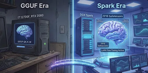
AI has evolved into a technology that can be effectively handled not just on massive cloud servers, but also on personal laptops or desktops. One of the key technologies enabling this change is the llama.cpp project, which centers around the GGUF (GPT-Generated Unified Format).
This article delves into the structural characteristics and design philosophy of GGUF and explores why this format has established itself as the standard in the local LLM ecosystem.
1. What is GGUF?

GGUF is the next-generation version of the GGML (Geroge Georgiev Machine Learning) format, designed by the llama.cpp team as a unified model file format.
While the original GGML merely stored tensors (Weights), GGUF presents a new level of architecture aimed at fully “packaging” a model.
Existing PyTorch .pth or Hugging Face .safetensors files solely store model weights. Therefore, the tokenizer, configuration files, and architecture information had to be loaded separately during the loading phase, and complex GPU and CUDA environment settings were essential.
In contrast, GGUF integrates weights + metadata + tokenizer + hyperparameters into a single binary file.
Thus, “moving a model” is no longer a complex task involving code or settings, but rather a simplified act of copying a single file.
The background of this design is the philosophy of ‘Complete Loadability’. In other words, the same GGUF file must operate identically on any hardware.
2. Key Technical Features of GGUF
GGUF is not just a format but a kind of system design paradigm for efficient local inference.
(1) Single File Structure
GGUF consolidates all data into a single binary file. This not only enhances file access (IO) efficiency but also simplifies model deployment.
Internally, the file consists of a header, metadata (Key-Value Dictionary), and tensor blocks.
Thanks to this structure, backward compatibility is maintained even when new fields are added. For instance, if new metadata like “prompt_format” is added, existing loaders will ignore it while the latest loaders will recognize it.
(2) Memory Mapping (mmap)
GGUF actively utilizes the OS-level memory mapping (mmap) feature. This allows only the necessary blocks to be immediately loaded without loading the entire file into RAM at once.
In other words, when running a 10GB model, the actual amount loaded into memory is limited to the “currently computed tensor.” This enables large models to run even in low-memory environments.
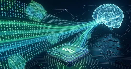
(3) Hardware Acceleration and Offloading
GGUF is fundamentally designed with CPU operations in mind, but when a GPU is available, some matrix operations can be offloaded to the GPU.
This structural flexibility allows GGUF to support three execution modes: CPU Only → Hybrid → GPU Assisted, providing a consistent performance profile across various platforms.
3. In-depth Understanding of Quantization
The biggest innovation of the GGUF format is its ability to “restructure (Quantize)” the numerical precision of models, rather than simply “saving” them.
Quantization refers to the process of compressing weights originally represented in floating-point format (e.g., FP16, FP32) to lower bit precision (e.g., 4bit, 5bit, etc.).
As a result, the file size and memory usage drastically decrease, while the semantic performance of the model largely remains intact.
(1) Meaning of Quantization Notation (Qn_K_M, Q8_0, etc.)
The names of the quantization methods used in GGUF are not just simple abbreviations, but rather codes reflecting the structure of the internal algorithms.
-
Q: Quantization (the type of quantization)
-
n: The number of bits used to represent a single weight (e.g., Q4 → 4 bits)
-
K: Refers to _K-Block Quantization_, which indicates a structure where matrices are divided into K-sized blocks for independent quantization.
For example, inQ4_K, the weight tensor is divided into blocks of size K, and the scale and zero-point are calculated separately for each block.
This allows reflecting local characteristics, resulting in much higher precision than simple global quantization. -
M: Refers to _Mixed Precision_.
Some tensors (especially Key/Value Projections and other vital parts) are stored with higher precision, while the rest are stored with lower precision.
This method applies precision differentially based on the structural importance of the model. -
0 (Zero): Denotes a “non-K” block structure. In other words, it refers to simple global scale quantization instead of K block units, which is the simplest structure but difficult for fine-tuning.
(2) Principles and Application Contexts of Each Quantization Method
| Quantization Type | Technical Description | Internal Mechanism | Recommended Use Environment |
|---|---|---|---|
| Q2_K | 2-bit quantization. Theoretically compresses 16 times. | Restores 4 values (2 bits × 16) based on scale for each block. | Extremely limited memory (Raspberry Pi, Edge devices). |
| Q3_K_M | 3-bit quantization + Mixed precision. | Expressed in 3 bits, using 4 bits or more for important tensors. | Low-spec laptops, embedded environments. |
| Q4_K_M | Practical standard for 4-bit quantization. | Balanced block scaling, quantization in K-sized groups. | General use (MacBook, gaming PCs). |
| Q5_K_M | 5-bit quantization, minimizing losses. | Provides finer scale intervals. | Environments with sufficient memory. |
| Q6_K | High precision quantization with minimal loss. | Scaling based on minimum and maximum values within each block. | For high-quality inference. |
| Q8_0 | 8-bit, simple quantization without blocks. | Closest to original performance. | For GPUs and high-performance workstations. |
> In general, Q4_K_M is considered the sweet spot for capacity vs. quality efficiency. This is due to the balance provided by the K block structure and the 4-bit compression, which align well with the current units of CPU/GPU computation (AVX, Metal, CUDA). |
4. Design Strengths of GGUF
-
Platform Independence: Inference can be performed with the same binary file on various hardware, including CPU, GPU, and Apple Silicon.
-
Loading Efficiency: Streaming loading based on mmap allows models in the gigabyte range to be run immediately.
-
Complete Reproducibility: Since the tokenizer and parameters are included within the file, the same GGUF file produces the same output anywhere, anytime.
-
Ecosystem Scalability: The format has been adopted as a standard across various tools like
Ollama,LM Studio,LocalAI, andllamacpp-python, centered aroundllama.cpp.
5. Limitations and Practical Considerations
-
Not suitable for training.
GGUF is an “inference optimization format” and does not maintain the data precision required for gradient backpropagation.
Thus, to fine-tune or re-train with methods like LoRA, one must convert back to the FP16 format. -
Speed limitations compared to GPU-specific formats.
Formats like EXL2, AWQ, and GPTQ leverage GPU matrix operations directly, resulting in faster token generation speeds.
However, these are mostly dependent on CUDA environments, with limited support for CPU/Metal and other general-purpose platforms.
GGUF’s design philosophy prioritizes universality and accessibility over speed.
6. Conclusion: GGUF as the “Standard Format for Personal AI”
With the emergence of GGUF, large language models are no longer the domain of research laboratories.
By achieving three pillars of inference efficiency in local environments, file unification, and hardware independence, GGUF has essentially established itself as the de facto standard for local LLMs.
If you want to run cutting-edge models like Llama 3, Mistral, or Phi-3 on your MacBook or regular PC —
the starting point is simply to download a GGUF format model.

There are no comments.