NumPy for Deep Learning Beginners: Why It Comes Before PyTorch

NumPy for Deep Learning Beginners: Why It Comes Before PyTorch

Why Deep Learning Beginners Should Start with NumPy

When you dive into deep learning books or courses, you’re usually introduced to frameworks like PyTorch or TensorFlow right away. But as you start building models, you often encounter these questions:

• "What exactly is a tensor?"
• "Why am I getting a shape mismatch error?"
• "I thought I could just concatenate batches this way…?"

Most of this confusion stems from jumping straight into a deep learning framework without a solid grasp of NumPy.

• PyTorch’s Tensor is almost identical to NumPy’s ndarray.
• Tasks such as data preprocessing, batch creation, and statistical calculations still rely on a NumPy‑style mindset.

So if you truly want to master deep learning, consider NumPy your essential foundational training.

What Is NumPy?

NumPy (short for Numerical Python) is a library that enables fast numerical computations in Python.

Key concepts:

• Multidimensional arrays (ndarray): the building blocks for vectors, matrices, and tensors.
• Vectorized operations: perform bulk calculations without explicit loops.
• Broadcasting: intelligently align arrays of different shapes for operations.
• Linear algebra: matrix multiplication, transposition, inversion, etc.
• Random module: data sampling, normal distributions, random initialization.

Almost every equation in deep learning boils down to vector and matrix operations, so NumPy is essentially the language of deep learning.

Python Lists vs. NumPy Arrays

Let’s quickly compare Python’s built‑in lists with NumPy arrays.

# Python lists
A = [1, 2, 3, 4]
B = [10, 20, 30, 40]

print(A + B)
# Output: [1, 2, 3, 4, 10, 20, 30, 40]  (concatenation)

The + operator for lists concatenates, not element‑wise addition.

import numpy as np

A = np.array([1, 2, 3, 4])
B = np.array([10, 20, 30, 40])

print(A + B)
# Output: [11 22 33 44]  (element‑wise addition)

NumPy’s + behaves like the mathematical operation we expect, and PyTorch tensors follow the same pattern.

Vectorization: Reduce Loops, Write Math‑Like Code

Deep learning code often emphasizes minimizing for loops in favor of vectorization.

Example: squaring every element.

Python List + for loop

values = [1, 2, 3, 4, 5]
squared = []
for x in values:
    squared.append(x ** 2)

print(squared)  # [1, 4, 9, 16, 25]

NumPy Vectorization

import numpy as np

values = np.array([1, 2, 3, 4, 5])
squared = values ** 2

print(squared)  # [ 1  4  9 16 25]

• Shorter code
• Reads more like mathematics
• Internally implemented in C for speed

PyTorch and TensorFlow tensors use the same vectorized NumPy‑style operations.

Broadcasting: Operate on Arrays of Different Shapes

Broadcasting automatically aligns arrays of different shapes for element‑wise operations.

Example: adding a constant vector to each sample.

import numpy as np

X = np.array([[1, 2, 3],
              [4, 5, 6]])   # shape: (2, 3)

B = np.array([10, 20, 30])  # shape: (3,)

Y = X + B
print(Y)
# [[11 22 33]
#  [14 25 36]]

NumPy expands B from (3,) to (1, 3) and then to (2, 3).

PyTorch follows the same rule:

import torch

X = torch.tensor([[1, 2, 3],
                  [4, 5, 6]])
B = torch.tensor([10, 20, 30])

Y = X + B
print(Y)

Understanding broadcasting in NumPy makes PyTorch tensor operations feel natural.

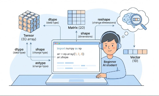
Vectors, Matrices, Tensors: Expressing Deep Learning with NumPy

Typical deep learning concepts in NumPy:

• Vector: 1‑D array → shape: (N,)
• Matrix: 2‑D array → shape: (M, N)
• Tensor: 3‑D or higher
• Example: a batch of grayscale 28×28 images
  • batch_size = 32 → shape: (32, 28, 28)

Simple matrix multiplication:

import numpy as np

# Input vector (3 features)
x = np.array([1.0, 2.0, 3.0])           # shape: (3,)

# Weight matrix (3 → 2)
W = np.array([[0.1, 0.2, 0.3],
              [0.4, 0.5, 0.6]])        # shape: (2, 3)

# Matrix product: y = W @ x
Y = W @ x
print(Y)  # [1.4 3.2]

This is essentially a single‑layer linear transformation. In PyTorch:

import torch

x = torch.tensor([1.0, 2.0, 3.0])   # shape: (3,)
W = torch.tensor([[0.1, 0.2, 0.3],
                  [0.4, 0.5, 0.6]]) # shape: (2, 3)

Y = W @ x
print(Y)

Familiarity with NumPy matrix operations translates directly to understanding tensor math.

How NumPy Connects to PyTorch

1. Tensors and ndarrays Are Cousins

• Both provide n‑dimensional arrays and vectorized operations.
• Functions like shape, reshape, transpose, sum, mean have similar names and behavior.

Many people use NumPy as a practice ground for PyTorch tensors.

2. Data Preprocessing Is Usually NumPy‑Style

Typical steps in a deep learning pipeline:

• Load CSVs, images, logs, etc.
• Convert to numeric form.
• Normalize, standardize, slice, shuffle, batch.

These tasks are often handled with NumPy + pandas.

import numpy as np
import torch

# Prepare data in NumPy
np_data = np.random.randn(100, 3)  # 100 samples, 3 features

# Convert to PyTorch tensor
tensor_data = torch.from_numpy(np_data).float()
print(tensor_data.shape)  # torch.Size([100, 3])

Conversely, you’ll frequently convert PyTorch tensors back to NumPy for post‑processing:

y = tensor_data.mean(dim=0)  # PyTorch tensor
y_np = y.detach().cpu().numpy()

Thus, in practice, NumPy and PyTorch constantly interoperate.

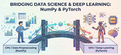
3. GPU Computation Is PyTorch, Concept Practice Is NumPy

• PyTorch tensors run on GPU (CUDA) and support automatic differentiation.
• NumPy is CPU‑only but is simpler for concept practice and debugging.

Typical workflow:

1. Prototype a formula in NumPy.
2. Once validated, port it to PyTorch.

Common NumPy Patterns in Deep Learning

1. Random Initialization & Adding Noise

import numpy as np

# Weight initialization (normal distribution)
W = np.random.randn(3, 3) * 0.01

# Add noise to input
x = np.array([1.0, 2.0, 3.0])
noise = np.random.normal(0, 0.1, size=x.shape)
x_noisy = x + noise

2. Data Normalization (mean 0, std 1)

X = np.random.randn(100, 3) * 10 + 50  # synthetic data

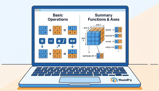
mean = X.mean(axis=0)
std = X.std(axis=0)

X_norm = (X - mean) / (std + 1e-8)

Normalization significantly impacts training stability and performance.

3. One‑Hot Encoding

num_classes = 4
labels = np.array([0, 2, 1, 3])

one_hot = np.eye(num_classes)[labels]
print(one_hot)
# [[1. 0. 0. 0.]
#  [0. 0. 1. 0.]
#  [0. 1. 0. 0.]
#  [0. 0. 0. 1.]]

PyTorch follows the same logic when creating one‑hot tensors.

4. Batch Splitting

X = np.random.randn(100, 3)  # 100 samples
batch_size = 16

for i in range(0, len(X), batch_size):
    batch = X[i:i+batch_size]
    # Think of feeding `batch` to a model here

This pattern maps directly to PyTorch’s DataLoader.

Key Points to Master When Studying NumPy

You don’t need to learn every feature. Focus on:

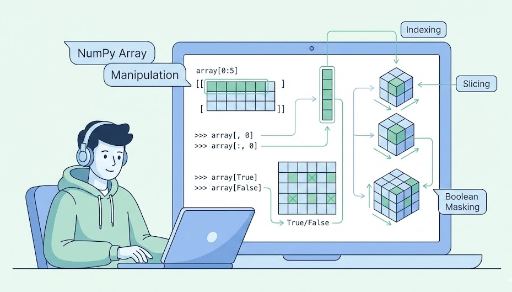
1. ndarray basics: np.array, dtype, shape, reshape, astype
2. Indexing & slicing: x[0], x[1:3], x[:, 0], x[:, 1:3], boolean indexing x[x > 0]
3. Basic arithmetic: +, -, *, /, **, comparison ops, np.sum, np.mean, np.max, np.min, axis
4. Linear algebra: matrix multiplication (@ or np.dot), transposition (x.T)
5. Broadcasting: scalar ops, patterns like (N, D) + (D,) or (N, 1)
6. Random utilities: np.random.randn, np.random.randint, np.random.permutation
7. PyTorch interop: torch.from_numpy, tensor.numpy(), shape consistency

Mastering these gives you a solid footing for PyTorch tutorials and tensor math.

Conclusion: NumPy Is the “Grammar” of Deep Learning

In summary:

• NumPy is a multidimensional array library for numerical computing.
• PyTorch’s Tensor is essentially a deep‑learning‑ready NumPy ndarray.
• By learning vectorization, broadcasting, and linear algebra in NumPy, you:
• Reduce shape errors
• Translate research equations into code more easily
• Enhance data preprocessing and analysis skills

If you want to understand deep learning from a mathematical and array‑operation perspective rather than just “how to use a framework,” NumPy is the perfect starting point.