NumPy Basics for Deep Learning: +, -, *, /, **, Comparisons, sum/mean/max/min, and axis
1. Why Start with Basic Operations?

In deep learning, what we ultimately do boils down to:
- Adding inputs and weights (
+) - Multiplying (element‑wise or matrix multiplication) (
*) - Applying non‑linear functions (
**,relu,sigmoid, etc.) - Computing loss and then either taking the average (
mean) or the sum (sum) of that loss
PyTorch’s tensor operations follow NumPy’s basic operation style exactly, so once you’re comfortable with NumPy’s feel, the deep‑learning formulas look much clearer.
2. Element‑wise Arithmetic: +, -, *, /, **
NumPy’s basic operations between arrays are element‑wise.
import numpy as np

x = np.array([1, 2, 3])
y = np.array([10, 20, 30])

print(x + y)   # [11 22 33]
print(x - y)   # [ -9 -18 -27]
print(x * y)   # [10 40 90]
print(y / x)   # [10. 10. 10.]
print(x ** 2)  # [1 4 9]
- One‑dimensional arrays of the same length are operated element‑wise
- Two‑ or three‑dimensional arrays follow the same rule: the same indices are combined
2.1 Operations with Scalars
Operations with a single number (scalar) are also natural.
x = np.array([1, 2, 3])

print(x + 10)   # [11 12 13]
print(x * 2)    # [2 4 6]
print(x / 2)    # [0.5 1.  1.5]
Adding or multiplying the same value to every element is common in deep learning for normalization, scaling, and bias addition.
PyTorch tensors behave the same way. Expressions like
x_t + y_t,x_t * 2, orx_t ** 2are almost identical.
3. Comparison Operations: >, <, >=, <=, ==, !=
Comparing two NumPy arrays yields a boolean array.
import numpy as np

x = np.array([1, 2, 3, 4, 5])

print(x > 3)   # [False False False  True  True]
print(x == 2)  # [False  True False False False]
This boolean array can be used as a mask to select elements or to count how many elements satisfy a condition.
Example:
x = np.array([1, -2, 3, 0, -5, 6])

mask = x > 0
print(mask)          # [ True False  True False False  True]

# Select positives
pos = x[mask]
print(pos)           # [1 3 6]

# Count positives
num_pos = np.sum(mask)   # True counts as 1, False as 0
print(num_pos)           # 3
In deep learning we often compute:
- Accuracy – the proportion of correctly predicted samples
- Loss that only includes positions meeting a certain condition
PyTorch follows the same pattern.
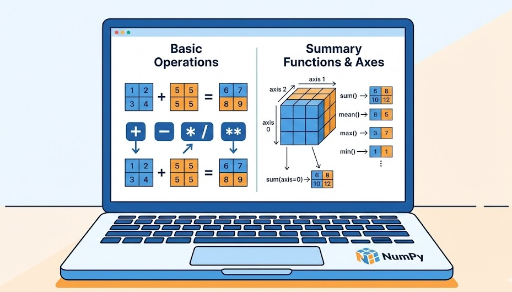
4. Aggregation Functions: np.sum, np.mean, np.max, np.min
4.1 Without an Axis: Whole‑Array Aggregation
The default form computes the sum, mean, max, or min over the entire array.
import numpy as np

x = np.array([1, 2, 3, 4])

print(np.sum(x))   # 10
print(np.mean(x))  # 2.5
print(np.max(x))   # 4
print(np.min(x))   # 1
The same applies to 2‑D or higher arrays.
X = np.array([[1, 2, 3],
              [4, 5, 6]])

print(np.sum(X))   # 21
print(np.mean(X))  # 3.5
In deep learning we use these for:
- The average loss over an entire batch or dataset
- Normalizing data by its overall mean and standard deviation
5. Understanding the axis Concept
axis tells NumPy which dimension to reduce along.
- No axis specified → compute over all elements
- Axis specified → reduce along that axis, leaving the remaining axes intact
5.1 A 2‑D Example
import numpy as np

X = np.array([[1, 2, 3],
              [4, 5, 6]])  # shape: (2, 3)
axis=0: Reduce along rows (column‑wise)
print(np.sum(X, axis=0))   # [5 7 9]
print(np.mean(X, axis=0))  # [2.5 3.5 4.5]
- Result shape:
(3,) - Each column is summed or averaged
- In deep learning, this is often used to compute feature‑wise statistics
axis=1: Reduce along columns (row‑wise)
print(np.sum(X, axis=1))   # [ 6 15]
print(np.mean(X, axis=1))  # [2. 5.]
- Result shape:
(2,) - Each row is summed or averaged
- In deep learning, this corresponds to sample‑wise totals or averages
5.2 Common Deep‑Learning axis Patterns
Suppose we have batch data:
# (batch_size, feature_dim)
X = np.random.randn(32, 10)  # 32 samples, 10‑dimensional features
- Feature‑wise mean
mean_per_feature = np.mean(X, axis=0) # shape: (10,)
axis=0collapses the batch dimension- Gives the mean of each feature across the batch
- Sample‑wise mean
mean_per_sample = np.mean(X, axis=1) # shape: (32,)
axis=1collapses the feature dimension- Gives the mean of each sample vector
5.3 Thinking About Image Batches
Consider a PyTorch‑style image batch (N, C, H, W).
NumPy can represent the same shape.
# N=32, C=3 (RGB), H=W=64
images = np.random.randn(32, 3, 64, 64)
Examples:
- Global pixel maximum
global_max = np.max(images) # scalar
- Channel‑wise mean (RGB)
# Reduce over batch, height, and width, keep channels
channel_mean = np.mean(images, axis=(0, 2, 3))  # shape: (3,)
This pattern is frequently used for channel‑wise normalization.
6. Aggregation + Comparison: Common Patterns
6.1 Accuracy Calculation
For binary classification:
import numpy as np

# Predicted probabilities (not logits)
pred = np.array([0.2, 0.8, 0.9, 0.3])
# Ground‑truth labels (0 or 1)
target = np.array([0, 1, 1, 0])

# Convert probabilities to class labels at 0.5 threshold
pred_label = (pred > 0.5).astype(np.int32)   # [0 1 1 0]

# Correct predictions
correct = (pred_label == target)             # [ True True True True]

accuracy = np.mean(correct)                  # True=1, False=0
print(accuracy)  # 1.0
The same logic applies in PyTorch.
6.2 Loss with a Mask
loss = np.array([0.1, 0.5, 0.2, 0.9])
mask = np.array([True, False, True, False])

masked_loss = loss[mask]      # [0.1, 0.2]
mean_loss = np.mean(masked_loss)
print(mean_loss)              # 0.15000000000000002
When you want to include only positions that satisfy a condition, the combination of masking + aggregation is very handy.
7. Summary: The Basic Operations Covered Today
- Arithmetic (
+,-,*,/,**) * Element‑wise by default * Works naturally with scalars - Comparisons (
>,<,>=,<=,==,!=) * Produce boolean arrays * Useful as masks for filtering, counting, or computing accuracy - Aggregation (
np.sum,np.mean,np.max,np.min) * Without an axis: whole‑array statistics * With an axis: reduce along a chosen dimension axisConcept *axis=0→ column‑wise (feature‑wise) in 2‑D *axis=1→ row‑wise (sample‑wise) * In deep learning, common shapes are(batch, feature)or(N, C, H, W)
Becoming comfortable with these basics lets you translate mathematical formulas into NumPy or PyTorch code almost instantly, making complex tensor operations feel natural.


There are no comments.